Controlled comparisons and detector results
The four pre-training arms, what each step between them isolates, the shared protocols, and the nuScenes and ONCE detection results with their uncertainty units stated.
The ladder
Four pre-training arms share one scaffold, one data split and one budget. Each step adds something to the left of the loss and nothing to the right of the encoder, so every comparison asks what a discarded part left behind.
- DirectNo added interfaceThe renderer reads the encoder output. Present-frame rays only.
- adds an interfaceone change
- ProjectionFeed-forward projectorAn action-free head sits between encoder and renderer. Present-frame rays only.
- adds recurrence and ego-motion conditioningtwo changes, bundled
- Recurrent ProjectionRecurrent, ego-motion conditionedTREND's head, with the future term switched off. Present-frame rays only.
- adds the future range lossone change
- ForecastingTREND's objectiveThe same recurrent head, supervised on present and future rays.
Only the encoder transfersEvery arm shares one scaffold, one dataset split and one pre-training budget. Everything the edges add lives to the right of the encoder and is deleted before fine-tuning, so each comparison asks what a discarded part left behind.
Reference. A randomly initialised detector, fine-tuned on the same data, marks where the whole ladder starts.
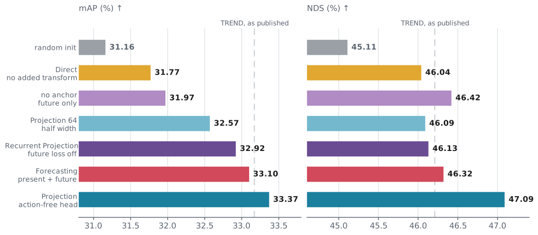
Side checks. Three further variants are run but not treated as coequal arms: a projector at half internal width, a head trained without the present-frame anchor, and a paper-like variant that reads the present loss from the encoder rather than through the head.
Reading the three steps as causal edges requires care, because they are not the same size.
Direct to Projection. One change. The renderer stops reading the encoder output and reads a four-block, 128-channel, action-free projector instead. Present-frame rays in both arms. Whatever separates them is the interface, not the objective.
Projection to Recurrent Projection. Two changes, bundled. The feed-forward projector is replaced by a recurrent step, and that step is conditioned on the ego action. Architecture and conditioning move together. A difference across this edge cannot be attributed to either one, and it is not treated as a single-factor result anywhere on this page.
Recurrent Projection to Forecasting. One change. The head is the same, the routing is the same, the budget is the same, and the future range loss is switched from off to on. This is the edge the headline question turns on, and it is the only edge that isolates future supervision.
Protocols held fixed
| nuScenes | ONCE | |
|---|---|---|
| Pre-training data | nuScenes sequences | ONCE raw sequences |
| Pre-training length | 48 epochs, 1114 iterations each | as released |
| Pre-training topology | global batch 24, 4 GPUs | as released |
| Pre-training runs per arm | 1 | 1 |
| Checkpoints read | pre-training epochs 12, 24, 36, 48 | pre-training epochs 12, 24, 36 |
| Detector | TransFusion-L | CenterPoint |
| Labelled subset | D160 | 20% |
| Fine-tuning schedule | 16x | 320 epochs |
| Fine-tuning batch | 4, one GPU | 48 |
| Metric | mAP, NDS, mAVE | AP@50 |
| Reference | random initialisation, same schedule | random initialisation, same schedule |
The fine-tuning batch topology was calibrated before it was used. On this few-shot subset the active variable is the per-GPU normalisation batch rather than the global batch: a single GPU at batch 4 reproduces the four-GPU, global-16 result to within about 0.15 mAP, while a single GPU at batch 16 sits about 0.5 lower. The registry protocol is therefore comparable with the published four-GPU one.
nuScenes, the full trajectories
Each arm is evaluated at the same four pre-training checkpoints under the same fine-tuning schedule. The trajectory is printed in full first: the matched-epoch comparison controls pre-training duration, while the peak comparison below is an exploratory best-attained summary.
| Pre-training epoch | Direct | Projection | Recurrent Projection | Forecasting |
|---|---|---|---|---|
| 12 | 31.52 / 46.13 | 31.32 / 45.28 | 31.54 / 45.38 | 31.55 / 45.06 |
| 24 | 31.77 / 46.04 | 31.88 / 46.15 | 32.14 / 45.97 | 33.10 / 46.32 |
| 36 | 32.12 / 45.74 | 33.37 / 47.09 | 32.92 / 46.13 | 32.38 / 45.80 |
| 48 | 31.85 / 45.28 | 33.35 / 46.71 | 32.75 / 46.65 | 32.65 / 45.50 |
mAP / NDS, TransFusion-L on nuScenes D160 at the 16x schedule, one fine-tuning execution per cell at a fixed seed, from one pre-training trajectory per arm. Random initialisation under the same schedule reaches 31.16 / 45.11, with a repeat at 31.08 / 44.49. Measured fine-tuning spread from seed repeats is about 0.4 to 0.6 mAP and 0.5 to 0.9 NDS, which is the band any two cells in this table have to clear before they mean anything.
Each arm at its own best checkpoint
The peaks are not aligned, so a best-attained summary is useful alongside the matched-epoch comparison. These checkpoints were selected after inspecting detection, however, and their peak differences should not be read as an unbiased estimate of an objective’s advantage.
| Arm | Peak mAP | at epoch | NDS there | Peak NDS | at epoch |
|---|---|---|---|---|---|
| Direct | 32.12 | 36 | 45.74 | 46.13 | 12 |
| Projection | 33.37 | 36 | 47.09 | 47.09 | 36 |
| Recurrent Projection | 32.92 | 36 | 46.13 | 46.65 | 48 |
| Forecasting | 33.10 | 24 | 46.32 | 46.32 | 24 |
Two readings come out of that.
No resolved future-loss advantage in this trajectory. Holding the recurrent head fixed and switching only the future term, each arm read at its own best checkpoint gives Forecasting +0.18 mAP and Recurrent Projection +0.33 NDS. Both sit inside the fine-tuning spread and they point in opposite directions. Reading the same pair at a fixed epoch would have given a different answer at every epoch: Forecasting is ahead by 0.96 mAP at epoch 24, level at epoch 12, and behind at 36 and 48. Even that epoch-24 figure does not survive matching on the fine-tuning seed, where the same checkpoint gives +0.35 and +0.18.
The interface does buy a peak. Direct and Projection both peak at epoch 36, so best against best and matched epoch are the same comparison here, and Projection is ahead by 1.25 mAP and 1.35 NDS.
The two arms differ only in whether a disposable head sits between encoder and renderer, the direction holds at epoch 48 as well (1.50 mAP, 1.43 NDS), and everything else is matched. The size is bounded rather than precise: a second execution of Projection at epoch 36, at the same seed, scores 32.85 and puts that gap at 0.73, and there is one pre-training trajectory per arm.
The same pair with repeats
The pair most often quoted from this work is the two strongest rows of that table, each with the fine-tuning repeated. Choosing a checkpoint per arm is still a choice made after seeing detection results, which is what the full trajectory above is printed to expose.
| Selected cell | mAP | NDS | mAVE | Executions |
|---|---|---|---|---|
| Forecasting, pre-training epoch 24 | 32.74 | 46.14 | 0.564 | 3 |
| Projection, pre-training epoch 36 | 32.94 | 46.70 | 0.540 | 3 |
Means over three fine-tuning executions from one pre-training checkpoint per arm. They are not three distinct seed labels: Forecasting is one execution at each of two seeds plus a repeat, and Projection is two executions at one seed plus one at another, so part of what these spreads measure is same-seed nondeterminism rather than seed variation. The two arms separate by 0.20 mAP, which is inside the spread of the executions themselves. The NDS and mAVE separation is more consistent: Projection has the higher NDS and the lower mAVE in all three of its executions, with no overlap against the three Forecasting executions in either column.
Both checkpoints were chosen after inspecting detection results. The trajectory table is the check on that: each of these two cells is a genuine peak with neighbours below it, rather than a single lucky point on an otherwise flat or still-rising curve.
Compute
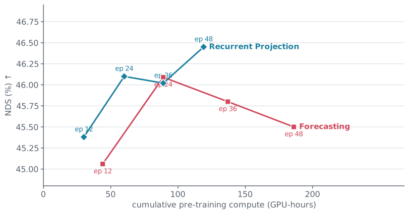
Pre-training cost is the other axis the comparison runs along, since the arms differ in what they render. It is accounted from per-iteration timestamps rather than job wall clock, over the same 1114 iterations per epoch and the same four-GPU topology, and the scope of each number is stated.
| Arm | GPU-hours to epoch 48 | Against Forecasting | Scope |
|---|---|---|---|
| Forecasting | 186.2 | reference | measured |
| Recurrent Projection, as intended | 119 | 36% less | estimated |
| Projection, as intended | 98 | 47% less | estimated |
| Projection at half internal width | 94.8 | 49% less | measured |
| Direct | 91.9 | 51% less | measured |
The two estimated rows exist for a specific reason. The completed Recurrent Projection and Projection runs carried a data-loading setting that made them load a second frame and render a future target on every step, whose loss was then multiplied by zero. That does not change the gradient either arm received, and the downstream results above are unaffected, but it means their wall clock measures work their objective does not require. The estimate prices the objective instead, from measured steady-state iteration time on the corrected configuration. The estimator was validated against three completed runs and lands 1.7% to 3.1% low on them; it is not used on the curriculum arm, where a first-epoch window cannot see a phase that begins at epoch 26.
Where the cost sits inside one iteration was measured directly on the Forecasting arm. Rendering accounts for about 82% of compute, the recurrent step for 6% to 15% depending on how many rendering passes backpropagate through it, and the encoder that fine-tuning keeps for about 2%. Replaying cached batches through the same loss module with one attribute flipped at a time puts the future rendering target at 1024 ms of a 2052 ms iteration, which is the measured origin of the roughly 50% saving.
ONCE, a second dataset and a second detector
ONCE contributes a different detector, a different metric and, unlike the nuScenes cells, three distinct fine-tuning seeds per cell.
The schedule was fixed before any arm was compared, by running the randomly initialised detector to convergence on this subset.
| Fine-tuning epochs | mAP | Vehicle | Pedestrian | Cyclist |
|---|---|---|---|---|
| 200 | 58.13 | 70.63 | 42.96 | 60.78 |
| 320 | 58.43 | 71.86 | 41.37 | 62.05 |
| 400 | 57.82 | 71.93 | 40.14 | 61.39 |
AP@50 on the ONCE 20% subset with CenterPoint. 320 epochs is the best scratch checkpoint, and training longer does not recover, so 320 is the schedule every pre-trained arm is fine-tuned under. The rung-to-rung spread of this ladder, about 0.3 to 0.6, is worth carrying into the next table.
| Arm | Pre-training epoch 12 | Pre-training epoch 24 |
|---|---|---|
| Forecasting | 58.30 ± 0.84 | 58.24 ± 0.42 |
| Recurrent Projection | 58.48 ± 0.53 | 58.25 ± 0.02 |
| Projection | 58.09 ± 0.28 | 58.21 ± 0.54 |
Mean and sample standard deviation over three distinct fine-tuning seeds (666, 42 and 2026), from one pre-training trajectory per arm. Random initialisation at the same schedule reaches 58.43 as a single run.
Paired across seeds, removing the future loss changes the result by +0.18 ± 1.36 at epoch 12 and +0.00 ± 0.41 at epoch 24. Replacing the recurrent head with the action-free projector changes it by +0.39 ± 0.42 and +0.03 ± 0.55. A single earlier execution had recorded 59.26 for Forecasting at epoch 12; it is the high realization of a cell whose three-seed mean is 58.30, and it does not represent a stable gain.
Epoch 36 is left out of that table on purpose. Two of the three arms have the full seed triple there, and the third has a single execution, so the three-arm comparison at that checkpoint is not comparable with the two above. Joining it to the curve would mix a three-seed mean with a one-run cell.
Uncertainty units, stated once
Every interval on this page is one of two things, and they are not interchangeable.
- Fine-tuning variation. Repeated fine-tuning executions, or distinct fine-tuning seeds, from a single pre-training checkpoint. Every error bar and every ± on this page is this.
- Pre-training variation. How much a result would move if the pre-training run itself were repeated. There is one pre-training run per arm, so this is never measured anywhere in this study.
The second is the variation most likely to matter for a claim about a pre-training objective, and its absence is the main limit on how far any of these results generalise.
The per-execution numbers behind every averaged cell on this page, and the full compute accounting, are recorded in the supplement.
Next Detection is one readout among several. Representation, motion probes and limits looks inside the discarded head and the retained encoder.