Detection head and row-selective evaluation

The end of a detector is regular. A shared feature row goes through many small prediction branches, the class scores are ranked, the best candidates are decoded into boxes, and rotated NMS removes overlaps. In VoxelNeXt this tail has six heads with six branches each, 36 branches in total, followed by top-k, decoding and NMS per head.

When DriveRT first ran the complete detector natively, decoding and NMS took about 7.3 ms of a 31 ms frame, and the raw prediction head another 4.6 ms. This page describes how those parts were reduced to under 1 ms together, and how the largest step turned from a detector-specific trick into a compiler rule.

All numbers are from one RTX 4060 Laptop GPU on nuScenes frames, recorded in the project notebook at the time of each change.

• 358 → 81decode kernel launches per frame
• 1.029 → 0.356 msdecode wall time per frame
• 7.6 mssaved over five frames by row-selective evaluation

Decoding on the device

The source detector decodes each head in Python: gather the selected rows, convert coordinates, exponentiate sizes, rebuild the rotation, filter by score and range, and remap classes. Every head reads its candidate count back to the host.

DriveRT fuses these steps into one CUDA launch per head and keeps candidate counts on the device, so the six heads need one count read at the end instead of up to twelve synchronizations. The sigmoid moved after top-k, because it does not change the ranking. Decoding and NMS went from about 7.3 ms to 1.7 to 2.0 ms.

Rotated NMS

Rotated NMS computes the overlap of every pair of candidate boxes. Three changes made it about 30 times cheaper without changing its result.

• Circle test. If the circumscribed circles of two boxes do not intersect, the boxes do not either, so the polygon intersection is skipped. Overlap time fell from 0.996 to 0.838 ms per frame.
• Polygon clipping. The overlap was computed by collecting up to 24 points and sorting them by angle. Clipping one rectangle by the other with the Sutherland-Hodgman algorithm reduced it from 0.856 to 0.304 ms.
• One thread per pair. The kernel used one GPU thread per candidate. With 248 candidates in the largest head, only 248 threads were active on the whole device. One thread per candidate pair reduced one call from 0.250 to 0.052 ms.

A tighter bounding-box test was also tried and made no measurable difference. The number of pairs reaching the clipping step was not the limit; the number of active threads was.

Top-k and a correction

Each head sorted every class logit, 28,000 to 45,000 values, to keep 500. Measured over the qualification frames, at most 248 logits per head pass the decoder’s score threshold. Selecting only those survivors, packing the six heads into one sort, reduced top-k from 0.349 to 0.053 ms. If a head has more survivors than the buffer holds, the exhaustive path runs instead.

The first version compared each logit against a cutoff computed on the host as log(t / (1 - t)), while the decoder compared the FP32 sigmoid against t. The two tests are equivalent in exact arithmetic but not in floating point. A later review found that near some thresholds the prefilter dropped candidates the decoder would have kept:

threshold   logit cutoff   dropped by prefilter
0.1         -2.197225      0
0.99         4.595120      3
0.999        6.906755      0 dropped, 125 kept extra

At the production threshold of 0.1 there was no disagreement, so the measured results stood. The kernel now evaluates the decoder’s own expression, 1 / (1 + exp(-logit)) > t, so both select the same set by construction. The extra exponential costs nothing measurable.

Batching the heads

After top-k was batched, decoding was limited by the host again: 0.53 ms of wall time for 0.25 ms of GPU work, issued from a loop over six heads. Candidate decoding, overlap masks, the greedy NMS pass and the final gather now run as one launch each, with the head as a block dimension.

decode wall time         1.029  ->  0.737  ->  0.530  ->  0.356 ms
decode GPU kernel time   0.817  ->  0.529  ->  0.252  ->  0.122 ms
decode kernel launches     358  ->    358  ->    180  ->     81

The first batched version indexed the gathered buffers with the candidate stride of 500, while those buffers are 83 wide. It produced wrong detections and a later CUDA fault, and the error disappeared when debugging prints forced synchronizations. A result that changes when something synchronizes usually points to an out-of-bounds write.

The prediction branches

Each of the 36 branches is a pointwise two-layer MLP over 128 channels. On the densest frame the hidden layers alone are 18 GFLOP, and the cuBLAS GEMMs for them already ran at 77% of the machine’s measured arithmetic ceiling. The remaining cost was data movement: 0.56 GB of hidden activations per frame, read and written four times, for the ReLU and 36 tiny output projections.

A fused kernel keeps each branch’s hidden values in thread-local registers and writes only the packed output. Isolated, the head went from 3.83 ms to 3.17 ms, and the complete detector improved by 0.15 ms on average over five measurements.

Four simpler fusions lost: one concatenated hidden GEMM (a 282 MB intermediate), a strided-batched GEMM, a cuBLASLt bias and ReLU epilogue per branch (host dispatch dominated), and fusing only the output projections.

Row-selective evaluation

The largest saving came from not computing most of the head.

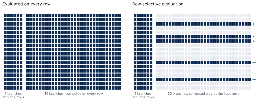
Of the 36 branches, six produce the class scores that top-k ranks. The other thirty produce box regression values, and the decoder reads them only at the few hundred rows top-k selected. Evaluating those thirty branches on every active row, up to about 15,000 rows, computes values nobody reads.

Query-based and center-based heads

Query-based heads avoid this by construction. TransFusion runs dense 3×3 convolutions to produce a class heatmap, keeps the top 200 positions as proposals, and runs its transformer decoder and its prediction layers (pointwise Conv1d) only on those 200 queries. The selection is written into the model.

Center-based heads compute every branch everywhere. CenterPoint’s regression branches are 3×3 convolutions over the whole BEV map, and its decoder reads them only at the top-k heatmap peaks. VoxelNeXt does the same with pointwise branches over its sparse rows.

Row-selective evaluation gives a center-based head the evaluation order of a query-based head without changing the model: the ranking branches run on every row, and the remaining branches run only on the rows the ranking keeps. For a query-based head the rule finds nothing to defer, because the model already does it.

The first implementation, in August, read which channels were ranking channels from the detector’s decoder. That worked for VoxelNeXt and nothing else. It was removed during the refactor and restored in September as a rule the compiler proves from the graph:

Evaluate a pure row-wise producer only on the rows its consumers select, when SSA and the canonical Operation semantics prove that this computes the same values at every row that is read.

A producer can be deferred only if all of the following hold on the graph:

1. it does not reach the ranking, so it cannot change which rows are selected;
2. every use of it is a gather along the row axis at an index produced by a proved selection;
3. every Operation on those paths is pure, row-wise and out-of-place;
4. the rows a mask keeps do not depend on the producer the mask is applied to;
5. it is not a graph output and has no other consumer.

A producer that fails any condition runs on every row, which is the ordinary evaluation. A failed proof costs speed and does not change results. The compiler records which Operation stopped the proof. Seven refusal cases are tested on renamed synthetic graphs: an escaping consumer, a graph output, a cross-row reduction, an in-place write, a value that reaches the selection, a gather with the wrong index chain, and a gather at an index no proved selection produces.

On the VoxelNeXt capture the rule partitions the branches into six ranking branches (5, 11, 17, 23, 29, 35) and thirty deferred ones. That is the same partition the August version used, now derived from the dataflow without any detector-specific input. The partition is stored in the Step’s Algorithm configuration as branch ordinals and proved again every time a Plan is loaded.

Results

With the input of the prediction region held fixed, the row-selective and eager evaluations are bit-identical on all five qualification frames: packed values at the selected rows, decoded candidates, NMS survivors, counts and final detections.

                 aggregate P50   launches   host syncs   copies   peak memory
row-selective       100.099 ms       1485           62       60      518.8 MB
eager               107.713 ms       1470           62       60      519.1 MB

Same Plan, same five frames, the partition declared or not, eight alternating blocks of 25 runs. Row-selective evaluation adds three launches per frame, for compaction and the deferred pass, and no host synchronization, because the selected indices and their count stay on the device.

Limits

• The proof is independent of the model. Execution is narrower: only the packed pointwise projection has a kernel that runs on a subset of rows. Any other producer family the proof accepts is refused at binding until it has such a kernel.
• CenterPoint has the same dataflow shape, but a 3×3 convolution reads neighbouring cells and is not row-wise, so the current rule keeps its branches dense. Supporting it needs a convolution kernel that evaluates only a list of output positions, and a proof condition for neighbourhood reads.
• The rule has been demonstrated on one detector, on one GPU.

The ranking branches

The six ranking branches still run on every row and took about 0.44 ms. A natural idea is to skip rows whose features are too small to produce a score above the threshold. The bound suggested first could not reject any row: even a row of zeros bounded above the threshold on five of six branches. A tighter bound that keeps the sign of the output weights is exact at zero and gives one cutoff feature norm per branch. A row can be skipped only if no branch can score, so the usable cutoff is the smallest of the six, 0.117, which corresponds to a row that is numerically empty. The expected pruning rate is close to zero, so it was not built.

Back to DriveRT · Sparse convolution in FP32